Matlab: Generate a pure tone with *.m file

To play a pure tone (sine wave) in Matlab, type the following code in a new file and save it as genTone.m:

function genTone(Fs, F, time)
t = 0:1/Fs:time;
y = sin(2*pi*F*t);
sound(y,Fs);
end

Now play sound in command

>> genTone(16000,100,0.5);
>> genTone(16000,1000,0.5);

The 3000Hz sound below will be wrong since it is greater than the 4000/2 = 2000 Hz Nyquist frequency.

>> genTone(4000,3000,0.5);

References:

how do i generate sound using MATLAB?
Chapter 2: Practical Audio Processing / tonegen.m (http://mcloughlin.eu/)

Matlab: Divide a speech utterance into 3 bands

>> load mtlb %Load the 'Matlab' speech / dimention: 4001x1
>> sound(mtlb,Fs); %Play the original sound
>> len = length(mtlb); %Number of points
>> time = [1:len]/Fs; %x-axis time vector / dimention: 1x4001
>> subplot(5,1,1);
>> plot(time,mtlb);
>> title('Original Speech');

>> Fco1 = 1000/(Fs/2); %Cutoff freq. 1
>> Fco2 = 2000/(Fs/2); %Cutoff freq. 2

>> [Bhpf, Ahpf] = butter(4,Fco2,'high'); %design a HPF

>> [Bbpf, Abpf] = butter(4,[Fco1 Fco2],'bandpass'); %design a BPF

>> [Blpf, Alpf] = butter(4,Fco1,'low'); %design a LPF

>> y_hpf = filter(Bhpf, Ahpf, mtlb); %get time domain result

>> y_bpf = filter(Bbpf, Abpf, mtlb); %get time domain result

>> y_lpf = filter(Blpf, Alpf, mtlb); %get time domain result

>> subplot(5,1,2);
>> y_reconstruct = y_hpf + y_bpf + y_lpf;

>> plot(time,y_reconstruct);

>> title('Reconstructed Speech');
>> sound(y_reconstruct,Fs); %Play the reconstructed sound

>> subplot(5,1,3);

>> plot(time,y_hpf);

>> title('HPF Speech');

>> sound(y_hpf,Fs); %Play the HPF sound

>> subplot(5,1,4);

>> plot(time,y_bpf);

>> title('BPF Speech');

>> sound(y_bpf,Fs); %Play the BPF sound

>> subplot(5,1,5);

>> plot(time,y_lpf);

>> title('LPF Speech');

>> sound(y_lpf,Fs); %Play the LPF sound

Result:

Matlab: Apply a LPF in the time and frequency using filter() and freqz()

The code below shows how to implement a 1000Hz Butterworth low pass filter using the filter() function in time domain and freqz() function in the complex frequency domain.

>> load mtlb %Load the 'Matlab' speech / dimention: 4001x1
>> sound(mtlb,Fs); %Play the original sound
>> len = length(mtlb); %Number of points
>> time = [1:len]/Fs; %x-axis time vector / dimention: 1x4001
>> subplot(3,1,1);
>> plot(time,mtlb);
>> title('Original Speech');

>> [b, a] = butter(3,1000/(Fs/2),'low'); %design a Butterworth filter

Time domain
>> y1 = filter(b, a, mtlb); %get time domain result directly % dimention: 4001x1
>> sound(y1,Fs); %Play the sound processed by filter()
>> subplot(3,1,2);
>> plot(time,y1);
>> title('filter()');

Frequency domain (Method 1)
>> mtlb_FFT = fft(mtlb); %transformed input signal / dimention: 4001x1
>> H = freqz(b, a, len, 'whole'); %filter transfer function / dimention: 4001x1
>> Y2_FFT = mtlb_FFT .* H; %filtered result in freq. domain = multiplication of transformed speech signal and the filter transfer function in the freq. domain. % dimention: 4001x1
>> y2 = ifft(Y2_FFT); %Inverse FFT to time domain % dimention: 4001x1
>> sound(y2, Fs);
>> subplot(3,1,3);
>> plot(time,y2);
>> title('freqz() and transform');

Frequency domain (Method 2)
>> mtlb_FFT = fft(mtlb); %transformed input signal / dimention: 4001x1
>> H = freqz(b, a, len); %filter transfer function / dimention: 4001x1
>> Y2_FFT = mtlb_FFT .* H; %filtered result in freq. domain = multiplication of transformed speech signal and the filter transfer function in the freq. domain. % dimention: 4001x1
>> y2 = ifft(Y2_FFT); %Inverse FFT to time domain % dimention: 4001x1
>> sound(abs(y2), Fs);
>> subplot(3,1,3);
>> plot(time,y2);
>> title('freqz() and transform');

Result:

References:

Matlab: Low pass filtered Chirp sound - Study EECC
Filter Applications (濾波器應用) - Audio Signal Processing and Recognition (音訊處理與辨識)
MATLAB: filter in the frequency domain using FFT/IFFT with an IIR filter - StackOverflow

Matlab: Low pass filtered Chirp sound

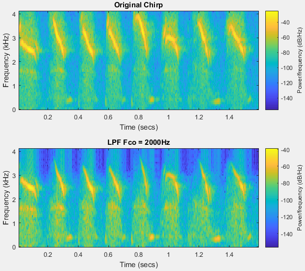
The Matlab commands below demonstrate a comparison of an original chirp sound and a processed sound using a 4th order Butterworth low-pass filter (LPF) with a 2000 Hz cutoff frequency.

>> load chirp
>> sound(y, Fs); %Play the sound
>> Fco = 2000; %Cutoff frequency
>> order = 4;
>> [b, a] = butter(order, Fco/(Fs/2), 'low'); %get numerator coefficients b and denominator coefficients a
>> ynew = filter(b, a, y); %get filtered result

>> sound(y,Fs); %play the original sound
>> sound(ynew,Fs); %play the filtered sound

>> x = [1:size(y)]/Fs; %x-axis scale (time)
>> subplot(2,1,1);
>> plot(x,y);
>> title('Original Chirp');

>> subplot(2,1,2);
>> plot(x,ynew);
>> title('LPF');
>> xlabel('sec');

Result:

Plot Spectrograms:

>> len = 100;
>> noverlap = 90;
>> NFFT = 128;
>> subplot(2,1,1);
>> spectrogram(y,len,noverlap,NFFT,Fs,'yaxis');
>> subplot(2,1,2);
>> spectrogram(ynew,len,noverlap,NFFT,Fs,'yaxis');

Result:

References

Filter Applications (濾波器應用) - Audio Signal Processing and Recognition (音訊處理與辨識)
Formant Estimation with LPC Coefficients - MathWorks Documentation
Matlab: Apply a LPF in the time and frequency using filter() and freqz() - Study EECC

Normalized Frequency 正規化頻率

frequency 頻率 unit: number of cycles/second (Hz) - f

normalized frequency 正規化頻率 = frequency (Hz) / sampling frequency (Hz) => fn = f / f_s

Example:

if f = f_s, then f_normalized = f/f_s = f_s/f_s = 1

if f = f_nyquist = f_s/2, then f_normalized = f/f_s = f_nyquist/f_s = (f_s/2)/f_s = 0.5

f_normalized = f/f_s => f = f_normalized × f_s

unnormalized frequency ω unit: radians/second (rad/sec)
normalized frequency ω_normalized = 2πf_normalized => f_normalized = ω_normalized/2π
=> f = f_normalized × f_s = ω_normalized× f_s/2π

其他表示符號(Loizou, 2013)：
 f = F/Fs

where

f = normalized frequency

F = frequency of signal

Fs = sampling frequency

頻率是每秒有幾個週期訊號

正規化頻率每個樣本有幾個週期訊號

例如取樣頻率16000Hz = 16000 samples/second

則8000Hz的正規化頻率是

(8000 cycles/second) / (16000 samples/second) = 0.5 cycles/sample

也就是每個樣本有半個週期

參考資料

What is actually Normalized Frequency?

P. C. Loizou, Speech Enhancement: Theory and Practice, 2nd ed., Boca Raton, FL, USA: CRC Press, pp. 15, 2013.

Matlab: play a sound file with command

To play a sound file with Matlab commands, type:

>> [y, fs] = audioread('filename.wav');
>> sound(y, fs)
>> plot([1:size(y)]/fs,y); %Plot waveform

>> xlabel('sec');

Matlab: record and play sound

To record sound with matlab, use audiorecorder() and getaudiodata()

In this example,
sample rate Fs = 8000
number of bits NBITS = 8
number of channels NCHANS = 1 = Mono

>> recorder = audiorecorder(8000,8,1);
>> record(recorder); //Say something
>> stop(recorder);
>> play(recorder);
>> data = getaudiodata(recorder, 'double');
>> sound(data, 8000);
>> plot([1:size(data)]/8000,data); %Plot waveform
>> xlabel('sec');

Waveform of Mandarin Chinese '1 2 3' (中文「一、二、三」的波形)

Reference:

McLoughlin, I. (2009). Applied speech and audio processing: with Matlab examples. Cambridge University Press. pp 7-10.