Matlab: Low pass filtered Chirp sound

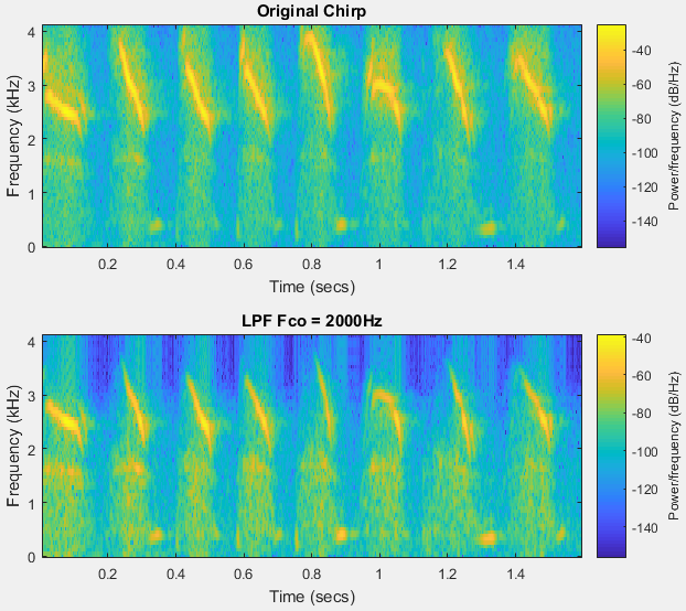
The Matlab commands below demonstrate a comparison of an original chirp sound and a processed sound using a 4th order Butterworth low-pass filter (LPF) with a 2000 Hz cutoff frequency.

>> load chirp
>> sound(y, Fs); %Play the sound
>> Fco = 2000; %Cutoff frequency
>> order = 4;
>> [b, a] = butter(order, Fco/(Fs/2), 'low'); %get numerator coefficients b and denominator coefficients a
>> ynew = filter(b, a, y); %get filtered result

>> sound(y,Fs); %play the original sound
>> sound(ynew,Fs); %play the filtered sound

>> x = [1:size(y)]/Fs; %x-axis scale (time)
>> subplot(2,1,1);
>> plot(x,y);
>> title('Original Chirp');

>> subplot(2,1,2);
>> plot(x,ynew);
>> title('LPF');
>> xlabel('sec');

Result:

Plot Spectrograms:

>> len = 100;
>> noverlap = 90;
>> NFFT = 128;
>> subplot(2,1,1);
>> spectrogram(y,len,noverlap,NFFT,Fs,'yaxis');
>> subplot(2,1,2);
>> spectrogram(ynew,len,noverlap,NFFT,Fs,'yaxis');

Result:

References

Filter Applications (濾波器應用) - Audio Signal Processing and Recognition (音訊處理與辨識)
Formant Estimation with LPC Coefficients - MathWorks Documentation
Matlab: Apply a LPF in the time and frequency using filter() and freqz() - Study EECC